
Blog
What are distributional shifts and why do they matter in industrial applications?
This article examines three types of distributional shifts: covariate shift, label shift, and concept shift, using a milling process simulation for downtime prediction. It emphasizes the need to monitor data distributions to maintain good model performance in dynamic environments like manufacturing.
What is distributional shift?
“Shift happens” – a simple yet profound realization in data analytics. Data distributions, the underlying fabric of our datasets, are often subject to frequent and often unexpected changes. These changes, known as “distributional shifts,” can dramatically alter the performance of machine learning (ML) models.
A core assumption of ML models is that data distributions do not change between the time you train a ML model and when you deploy it to make predictions. However, in real-world scenarios, this assumption often fails, as data can be interconnected and influenced by external factors. An example of such distributional shifts is how ML models went haywire when our shopping habits changed overnight during the pandemic.
There are three primary types of distributional shifts: covariate shift, label shift, and concept shift. Each represents a different way in which data can deviate from expected patterns. This article explores these forms of distributional shifts in a milling process, where we assess the performance of ML models in a downtime prediction task.
Simulation setup
In order to illustrate the impact of distributional shifts in industrial settings, we set up a simulation for predicting machine downtime in a milling process. Our goal is to determine whether a machine will malfunction during a production run, which helps anticipate capacity constraints proactively.
Our primary variable of interest is “Machine Health,” a binary indicator where:
- Machine Health = 0 indicates a machine breakdown.
- Machine Health = 1 indicates the machine is running flawlessly.
Several covariates are considered to be potential predictors of Machine Health. These are:
- Operating Temperature (°C)
- Lubricant Level (%)
- Power Supply (V)
- Vibration (mm/s)
- Usage Time (hours)
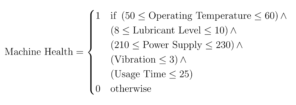
The relationship between these covariates and the Machine Health is encapsulated in the below ground-truth function. This function dictates the conditions under which a machine is likely to fail:
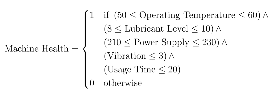
Here’s a breakdown of the formula:
- If the Operating Temperature is below 50°C or above 60°C there is a machine breakdown
- If the Lubricant Level is below 8% or above 10% there is a machine breakdown
- If the Power Supply is below 210V or above 230V there is a machine breakdown
- If the Vibration is above 3 mm/s there is a machine breakdown
- If the Usage Time is above 20 hour there is a machine breakdown
To simulate this process, we generate data for 1000 production runs based on the above ground-truth function. A Random Forest classifier is then trained on this data. Note that the above ground-truth function is assumed to be unknown when making predictions. The classifier’s task is to predict potential breakdowns in future production runs based on the observed covariates.
No shift
Moving forward with our simulation, we now introduce a “no shift” scenario to evaluate the robustness of our trained Random Forest classifier under conditions where there is no distributional shift. We generate an additional 250 production runs, which serve as our test set during model deployment. These new runs are created under the same conditions and assumptions as the initial 1000 production runs used for training the model. It’s important to note that we are deliberately not introducing any changes to the underlying data distribution in this particular example. This allows us to evaluate how well the classifier performs when the test data closely mirrors the training data.
Below, we present a comparative visualization of the variables’ distributions between model training and model deployment (i.e., predicting the Machine Health for the test set). The figure offers a clear perspective on the consistency of data across both the training set and the test set. By keeping the distribution of Operating Temperature, Lubricant Level, Power Supply, Vibration, and Usage Time identical to the training phase, we aim to replicate the ideal conditions under which the ML model was originally trained.

In this no-shift scenario, our Random Forest classifier achieves an accuracy of 100%. This result is not surprising, as the test data was created with the same data generation function as the training data. The classifier effectively recognizes and applies the patterns it learned during training, which leads to flawless predictions. This no-shift scenario serves as a benchmark against which we will compare the model’s performance in subsequent scenarios involving different types of distributional shifts.
Covariate shift
We now explore the concept of covariate shift, a common challenge in the application of ML models in real-world settings. Covariate shift occurs when there is a change in the distribution of the covariates between model training and model deployment (Ptrain(x) ≠ Ptest(x)), while the way these covariates relate to the outcome remains the same (Ptrain(y|x) = Ptest(y|x)).
To demonstrate the effect of covariate shift, we simulate a scenario for our simulated downtime prediction task. We assume that our factory has received a substantially large order, which requires us to extend the Usage Time on our milling machine. This increase in Usage Time naturally leads to higher Operating Temperatures and a decrease in Lubricant Levels, which alters the data distribution for these specific covariates.
We simulate an additional 250 production runs under these modified conditions. This new data serves as our test set, which now differs in the distribution of key covariates (Operating Temperature, Lubricant Level, and Usage Time) from the original training set. Below, we visualize the differences in distributions of these covariates between model training and model deployment.
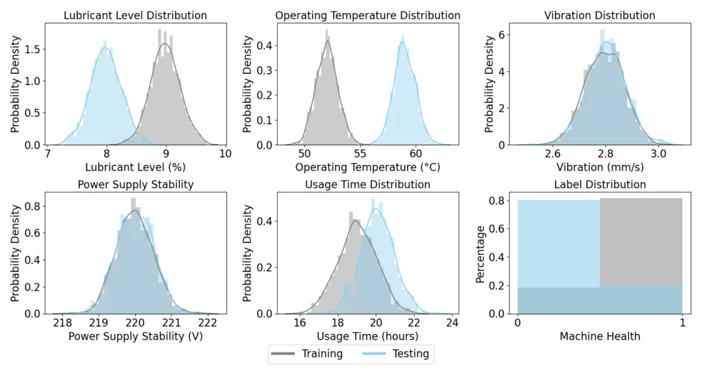
When applying our previously trained Random Forest classifier to this new test set, we observe a significant drop in accuracy, with the model achieving 72% accuracy. This decrease from the 100% accuracy seen in the no-shift scenario clearly illustrates the challenges posed by covariate shift. The model, trained on data with different covariate distributions, struggles to adapt to the new conditions, which leads to a noticeable reduction in its predictive accuracy.
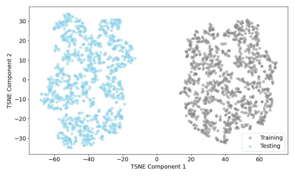
Our results demonstrate the importance of monitoring covariate shifts in dynamic environments. Detecting these shifts is crucial, but in high-dimensional scenarios where multiple covariates may shift together, tracking individual features becomes a challenging task. Compared to our simulated environment, real-world applications may involve hundreds of covariates. To address this high complexity, one can turn to dimensionality reduction techniques like t-SNE (t-distributed Stochastic Neighbor Embedding).
t-SNE is a nonlinear dimensionality reduction technique that can be used to visualize high-dimensional data in a low-dimensional space. Such visualizations provide a clear perspective on how the data is distributed across different dimensions. The t-SNE plot below demonstrates this for our milling process, where the five covariates are reduced to two dimensions, while aiming to retain most information. It can be observed that the training data (gray) and testing data (blue) form distinct clusters, which visually indicates a covariate shift. This separation highlights the need to reassess our model’s predictive reliability under these new conditions.
Label shift
Next, we delve into label shift, another form of distributional shift. Label shift occurs when the distribution of the labels changes between modeling training and model deployment (Ptrain(y) ≠ Ptest(y)), while the conditional distribution of the covariates given the label remains constant (Ptrain(x|y) = Ptest(x|y)).
To illustrate an example of label shift, we simulate a test set for another milling machine, which, compared to the first milling machine, is more prone to breakdowns. This change increases the likelihood of machine failures, thus altering the distribution of the Machine Health label. We generate data for 250 production runs under these new conditions, where the probability of breakdowns (Machine Health = 0) is higher than in our initial training dataset.
In the figure below, we visualize the distribution of the covariates and the Machine Health label across the training and testing data sets. The visual comparison clearly shows a shift in the label distribution, with a substantially higher frequency of breakdowns in the test data. Note that there is also a shift in the Vibration covariate. Here it is assumed that Vibration is a symptom of machine breakdowns. Following the definition of a label shift, the causal effect here is from the label (i.e., Machine Health) to the covariate (i.e., Vibration).
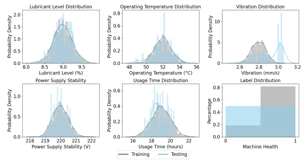
We now apply the Random Forest classifier to this new dataset and find that the model achieves an accuracy of 86%. This result marks a clear decrease from the perfect accuracy observed in the no-shift scenario. Despite being trained on data where breakdowns were frequent, the model now faces a scenario where breakdowns are more common, which deteriorates its predictive accuracy.
This example highlights the need for models to be adaptable to changes in the label distribution, especially in dynamic environments where the frequency or nature of the target variable can vary over time. Detecting label shifts is more straightforward than identifying covariate or concept shifts. Regular examination of the class label distributions is a key approach to ensure they accurately represent the deployment environment.
Concept shift
Concept shift, or concept drift, is the third form of distributional shifts that we will investigate. It is characterized by changes in the underlying relationship between covariates and labels over time (Ptrain(y|x) ≠ Ptest(y|x)). Such shifts mean that a model’s predictions may become less accurate as the learned relationships become outdated in the face of new data dynamics.
To illustrate concept shift, we introduce a new context to our simulation. Specifically, we assume that following multiple machine breakdowns we introduced a new maintenance routine for our milling machines. This new routine affects the relationship between our covariates and the Machine Health label. With better maintenance, the milling machines can operate for longer periods without breakdowns, thereby altering the way the Usage Time covariate relates to the Machine Health label. The new maintenance routine adjusts our ground-truth formula as follows:
We simulate 250 production runs with the updated maintenance routine for the test set. The distributions of the covariates and the Machine Health label in the training and testing datasets are depicted below. This deployment setting reflects the new reality where the relationship between the Usage Time and Machine Health has shifted due to improved maintenance practices. Despite similar covariate distributions, it can be observed that the number of machine breakdowns has been significantly reduced.
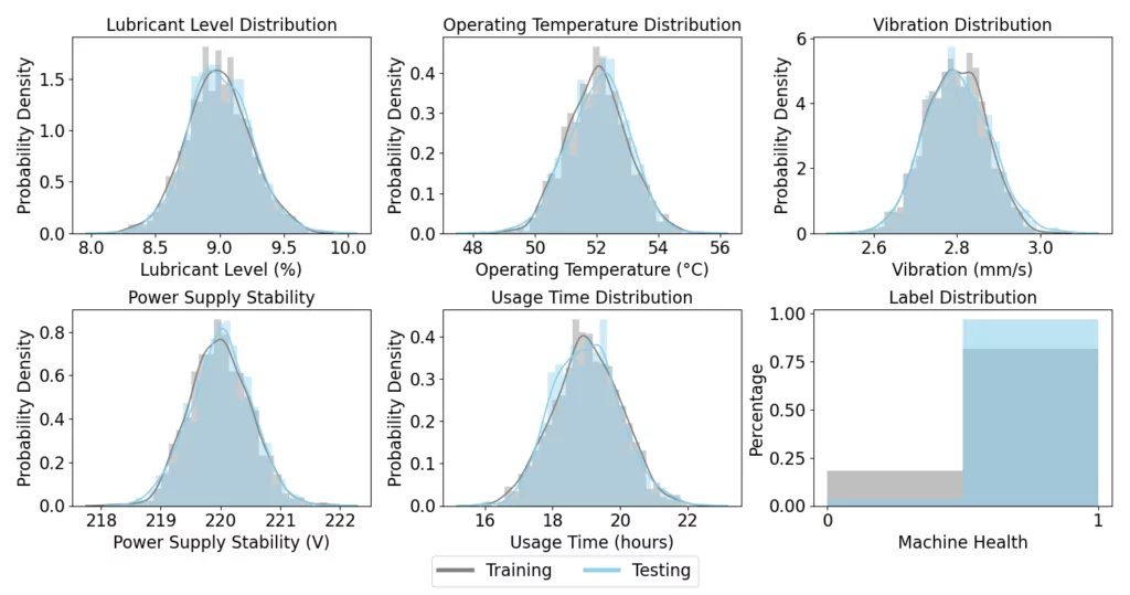
The Random Forest classifier, which was initially trained under different operational conditions, now encounters data where the ground-truth relationship between variables has fundamentally changed. When applying the classifier to this new data, we observe an accuracy of 84%. This decrease from the no-shift scenario demonstrates the impact of concept shift on the model’s predictive accuracy.
Detecting concept drift is challenging because it can often appear gradually. A general strategy to detect this form of distributional shift is to systematically monitor the performance of ML models over time. This continuous assessment helps in pinpointing when the model’s predictions start deviating from expected outcomes, suggesting that the underlying relationships between covariates and labels might have changed.
Conclusion
This article highlights a fundamental challenge in real-world applications of ML: data is constantly changing, and models must be adapted accordingly. We conducted simulations of machine downtime in a milling process to showcase the challenges posed by covariate, label, and concept shifts. In an ideal no-shift scenario, our model achieved perfect accuracy, but this quickly changed under real-world conditions of shifting data distributions.
Conventional ML models, like Random Forests, are increasingly used for industrial applications. While these methods have been made accessible to a wide audience through open source libraries (e.g., scikit-learn), they are often blindly deployed without fully assessing their performance in dynamic environments. We hope this article prompts practitioners to prioritize model monitoring and regular model retraining as key practices for preserving long-term model performance.
Readers interested in learning more about distributional shifts in manufacturing can find a case study from Aker Solutions in our recent paper, published in Production and Operations Management.